Things are really getting exciting now! That's great to start diving into some code, working on real data to solve a real business case. We will be mainly highlighting in this post the key aspects to be cautious about when kicking-off a new machine learning project.
/!\ Note that the code for this section is available on Aurelien Geron's github. It run's on top of Jupyter. All the commands and plots are available there for greater details on how he's using key frameworks (sk-learn, pandas, numpy..) and data vizualisation commands (matplotlib).
Link: https://github.com/ageron/handson-ml/blob/master/02_end_to_end_machine_learning_project.ipynb.
Project Context
It deals with modeling California Housing Price. The objective is to be able to build pricing predictions for new houses and eventually decide if it worths making investments. But before jumping into coding a model, one should observe few preliminary checks:
- Prepare a Machine Learning checklist, having at sight the guardrails to avoid the common pitfalls that we introduced in the previous article.
- Always experiment with real data when you jump in the field rather than artificial datasets. And hopefully, there are plenty of them out there: Amazon AWS datasets, Kaggle, dataportals.org, quandl.com, ...
- Frame the problem: it is a key pre-requisite to clarify expectations, ensuring what our model will provide as a business value and the desired output (prediction vs classification..). You wouldn't like to spend months building a model making it capable of providing a precise numeric predictions (i.e 5231$ per square feet), when the consuming component (team) down the data pipeline, can be satisfied with an estimate value (i.e 5000$) that they would map to either low, medium or high. In the end, this will allow you to identify what kind of model will work best for this problem, is it supervised, unsupervised or reinforcement learning ?
In this case, it's a supervised learning problem. Obviously we have enough data with multiple features to consider (district population, median housing price, median income, ..), making it a typical multivariate regression problem. Note that if the data is huge, we can either split the batch learning work across multiple servers (using MapReduce), or use an online learning technique instead.
Python environment
Main things to consider when setting up the Python dev environment:
- Create a dedicated workspace
- Create an isolated environment (i.e using Anaconda or virtualenv): prevent collisions with other project dependencies.
- Install key dependencies, mainly Jupyter, Numpy, Pandas, Matplotlib & Scikit-Learn: a best practice is to use a requirement.txt file, including all the dependencies the project will need. Then install everything using pip.
Test Set preparation
When you build a new ML project, you want to start by extracting a test set first, following these key steps :
- Automate the process to fetch your model training data: either downloading it from on of the databanks on net, or batching multiple data-sources (databases, spreadsheets..). That will allow you to refresh your data source with less effort over time.
- Take a quick look to the data structure: to get a first understanding on the data (types, features, size, number of non-null values, capped values..) using frameworks like Pandas (i.e pandas.read_csv(..), pandas.info(), ..) or through vizualisation by plotting the data through Matplotlib (detecting if some features are tail heavy, scales, ..)
- Build a representative test set: After a 1st quick overview of your data, you want to jump quickly into creating a Test Set using randomly 20%, and Numpy is the right library to use for this. But picking up randomly 20% is not perfect, cause each time you would run the program, you will end-up with a different set, using numpy random "seed" method migiates it, ensuring that we always pick the same shuffled indices. Both methods might break next time you fetch an updated dataset, since records might end-up at different indices. Another solution is to compute a hash value for each record identifier and keep only the two last bytes of the hash putting any value lower to 51 (~20% 256) within the test set. Skikit-learn provides few functions to split datasets (train_test_split from sklearn.model_selection, StratifiedShuffleSplit class). Lastly, the test set should be representative of the data distribution following a stratified sampling approach. This is to ensure that our test set is representative of the various categories in the whole dataset. Also ensure that you are using or adjusting a feature to come up with different strata (not too many), having each stratum being large enough.
- Select the performance measure for our Mode: RMSE (Root Mean Square Error) is the most popular one. However, in some context you may prefer to use another one, such as the MAE (Mean Absolute Error) in case there are many outlier districts. These are both specific euclidian norms (l2 & l1), having as a general rule to consider using a low value for the norm (i.e l1 instead for l2) when you have a distribution with outliers that are key for making the decision.
It's critical to spend time thinking properly about how the test set will be split so that it is representative of the key strata in your overall dataset. This is often neglected part of Machine Learning project.
You don't want to spend too much time analyzing you full dataset and coming with a model at this stage, which might be source of data snooping biais. Indeed, as humans, our brain is an amazing pattern detection system, which means that it is highly prone to overfitting.
Vizualizing Data
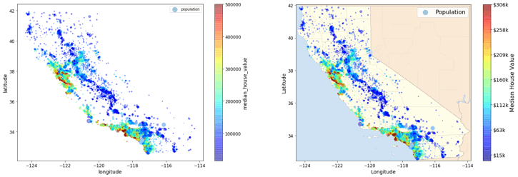
Now that you have defined the test set, It is the time to get a little more depth and insights by visualizing the training data set. Plotting it against the different features will help you get important insights, identifying key data patterns and ideally the kind of algorithms to use for solving our problem. For example, plotting the data of California housing prices using the geographical attributes (lon, lat), can help you spot high-density areas (i.e San Diego, Los Angeles and the Central Valley), also the scattered plot looks like San Francisco.

Looking at this, we can easily spot that there's a correlation between the housing prices and the location (i.e close to the ocean) and the population density. This gives us a hint that it might be relevant to use a clustering algorithm to detect main clusters and add a feature to measure the proximity to the cluster centers, and probably the proximity to the ocean.
Evaluate how far the different attributes are correlated, which will help you identify which features have to more influence and sensitivity on each other, also data quirks that you want to clean-up. Then focusing the model on most important features or even by create new one as the result of combining some attributes (i.e population per household).
Automate data transformation
Automating the data source transformation is one of the most important steps at this stage:
- Cleaning values: replacing null values with feature mean value for instance leveraging the Imputer class available in scikit-learn preprocessing module (sklearn.preprocessing)
- Removing or toggling some features to adjust the model complexity, hence mitigating underfitting/overfitting situation.
- Scaling numeric values to reduce the variance: prediction models usually work best when the features are either normalised or standardised to a lower range of values. Scikit-learn provides utility classes for this (i.e StandardScaler, MinMaxScaler)
- Combining some features using the TransformerMixin in sklearn.base
The more you automate these data preparation steps, the more combinations you can automatically try out, making it more likely that to find a great combination for your model, finally saving you a lot of time in the long run. It's recommended to create a script that will automatically transform the data before feeding it to the training algorithm, this will allow you to:
- easily reproduce these transformations on any dataset
- gradually building a library of transformation functions to reuse in new projects
- gain ability to combine different transformations quickly and identify which ones provide the best performance.
Once you have automated these different transformations, you can plug them all together using sklearn.pipeline and test them with different hyper-parameters on the training set. You want to test quickly few algorithms to identify the most promising ones (i.e LinearRegression, DecisionTree, RandomForest,..), based on their performance (training set vs cross-validation set).
Going further, both GridSearchCV or RandomizedSearchCV (in sklearn.model_selection module) can help you automate quickly the combination of multiple parameters to find the best parameters that will give the best prediction accuracy and the best estimator/algorithm. Once identified, you can finally assess your final algorithm on the test set as a last security net before deploying your model to production.
Last but not least, you will often want to review your data quality, otherwise the model will tend to stale. As data evolves over time, it can introduce sudden breakage or performance degradation. Hence, it is advised to regularly train the model on fresh data while reviewing system's input data quality.

